Edited by Markdown

Refered from: John Ladd, Jessica Otis, Christopher N. Warren, and Scott Weingart, “Exploring and Analyzing Network Data with Python,” The Programming Historian 6 (2017), https://programminghistorian.org/en/lessons/exploring-and-analyzing-network-data-with-python.

只是一个笔记，细节要看原文。

用python探索和分析网络数据

Table of Contents

1. 目标和要求
2. [数据准备 和 NetworkX 安装](#数据准备 和 NetworkX 安装)
3. 获取数据和基本的操作
4. 进一步分析
   • [添加属性](#Add attributes)
5. 网络度量分析
   • The Shape of the Network
     • 最短路径
     • 找出最大component 并生成子图
     • triadic closure
   • Centrality
     • 度数
     • 特征值中心性
     • 介数中心性
6. 社区发现
7. 导出数据和做结论

目标和要求

**Goals:**做完这里的步骤，你将得到如下技能：

• 使用Python的NetworkX 包来分析一个网络。
• 通过分析一个humanities network data来得到以下几点：
  • 网络结构和path length
  • 找到重要的或中心的节点
  • 找到社区和subgroups
• 通过量化网络分析的方法，你将可以回答像这样的问题：
  • What is the overall structure of the network?
  • Who are the important people, or hubs, in the network?
  • What are the subgroups and communities in the network?

说明：主要是关注网络中的统计信息，而不关注可视化，其实本文是对可视化问题的补充。如果你感兴趣可视化，可先参考link

要求：

• 先看过“从诠释学到数据到网络:历史来源的数据提取和网络可视化”link
• python3 , 而不是 python2, (unix-based的操作系统，比如 OSX, 会预装python2)，有问题可以link
• 装了pip 包管理工具

如果python2和python3同时装了的，那每次命令中 python / pip时，都要指明成： python3 / pip3，参考：装python 和 work with pip

我们的例子：朋友社会 在Facebook上有朋友之前，有朋友协会，被称为贵格会（Quakers）。贵格会教友会于17世纪中叶在英格兰成立，是新教基督徒（Protestant Christians），他们反对英国官方教会，提倡广泛的宗教宽容，更喜欢基督徒所谓的“内在光明”和良心，而不是国家强制的正统教义。贵格会信徒的数量在17世纪中后期迅速增长，他们的成员遍布不列颠群岛、欧洲和新大陆的殖民地——尤其是宾夕法尼亚，贵格会领袖威廉·佩恩创立了贵格会，是四位作者的故乡。

由于学者们一直将贵格会的成长和持续时间与他们的网络的有效性联系在一起，所以本教程中使用的数据是17世纪最早的贵格会成员的名单和关系。这个数据集来源于《牛津国家传记词典》和正在进行的弗兰西斯·培根六度计划，该计划正在重建早期现代英国(1500-1700年)的社会网络。

数据准备 和 NetworkX 安装

The file quakers_nodelist.csv is a list of early modern Quakers (nodes) and the file quakers_edgelist.csv is a list of relationships between those Quakers (edges). To download these files, simply right-click on the links and select “Save Link As…”.

networkx

pip3 install networkx

modularity

pip3 install python-louvain==0.5

Recently, NetworkX updated to version 2.0. If you’re running into any problems with the code below and have worked with NetworkX before, you might try updating both the above packages with pip3 install networkx --upgrade and pip3 install python-louvain --upgrade.

你准备好了networkx 和 modularity package后，就可以开始写code了。 如果遇到pyCharm环境中找不到module，参考如下：

pyCharm can manage python modules, third-party module packages easily. Do the steps:

• pyCharm » Preference, search ‘interpreter’, click “Project Interpreter”
• click ‘+’, enter the package name, click ‘Install Package’

获取数据和基本的操作

导入我们需要的4个包，其中2个是刚刚安装的，2个是python built-in package.

    import csv
    from operator import itemgetter
    import networkx as nx
    import community #this is from python-louvain

下一步就是从文件导入数据，通常导数据进来比较费code，比analysis还要费。打开文件，读取edge list 和 node list：

with open('quakers_nodelist.csv', 'r') as nodecsv: # Open the file                       
    nodereader = csv.reader(nodecsv) # Read the csv  
    # Retrieve the data (using Python list comprhension and list slicing to remove the header row, see footnote 3)
    nodes = [n for n in nodereader][1:]                     

node_names = [n[0] for n in nodes] # Get a list of only the node names                                       

with open('quakers_edgelist.csv', 'r') as edgecsv: # Open the file
    edgereader = csv.reader(edgecsv) # Read the csv     
    edges = [tuple(e) for e in edgereader][1:] # Retrieve the data

print(len(node_names))
print(len(edges))

Appendix afterwards 2019-11-12: import graph by csv file:

edges_csv_path = 'net_data/karate_club/graph_karate_edges_label1.csv'  # import graph by csv file
net_data = open(edges_csv_path, "r")
next(net_data, None)  # skip the first line in the input file
G = nx.parse_edgelist(net_data, delimiter=',', create_using=nx.Graph(),
                      nodetype=int, data=None)  # data=(('weight', float),)
# import matplotlib.pyplot as plt
# nx.draw_networkx(G, with_labels=True)  # draw the graph, simplest way.
# # nx.draw_spring(G, with_labels = True)
# plt.show()

# output to csv: (write/output the graph data/edges into csv file)
nx.write_edgelist(G, 'netME.csv', delimiter=',', data=False)   # note data = False will not write '{}'

draw graph with position dictionary:

import matplotlib.pyplot as plt
import networkx as nx

G = nx.les_miserables_graph()    # use the les_miserables_graph()
pos = nx.spring_layout(G, k=0.42, iterations=100)    # more: networkx.drawing.layout.*
nx.draw(G, pos, with_labels=True)
# nx.draw_spring(G, with_labels = True)  #replaced by above 2 lines
plt.show()
print(nx.info(G))

NetworkX 基础，创建Graph

Now you have your data as two Python lists: a list of nodes (node_names) and a list of edges (edges).

1. create Graph object:

 G = nx.Graph()  #create a Graph obj G, with nothing in it.
 # add lists of nodes and edges like below:
 G.add_nodes_from(node_names)
 G.add_edges_from(edges)

这是一种方法，更多的向Graph对象填值的方法要看networkX官方文档

最后，你可以用info函数看看你刚创建的Graph的基本情况：

print(nx.info(G))

现在应该能看到这个Graph的一些基本的，表面的情况，但还远远不够。。

邻接矩阵的生成

from networkx import karate_club_graph, to_numpy_matrix
zkc = karate_club_graph()
order = sorted(list(zkc.nodes()))  # order = [0,1,2,...]
A = to_numpy_matrix(zkc, nodelist=order)   # 输入一个nx.graph, this shows how to generate its adj_Matrix
# degree matrix: 度矩阵的生成
D = np.array(np.sum(A, axis=0))[0]
D = np.matrix(np.diag(D))

进一步分析

Add attributes

光有了Nodes, & edges还不够，还可以用networkx添加attributes到nodes&edges. 开始创建的list，nodes包含了你需要的信息。NetworkX provides two convenient functions for adding attributes to all of a Graph’s nodes or edges at once: nx.set_node_attributes() and nx.set_edge_attributes(). 但使用2者之前，要求你的数据是在python dictionary里。意思是，name是keys；attributes是values.每个attribute都要创建一个dictionary，用花括号{}:

hist_sig_dict = {}
gender_dict = {}
birth_dict = {}
death_dict = {}
id_dict = {}

Now we can loop through our nodes list and add the appropriate items to each dictionary.

for node in nodes: # Loop through the list, one row at a time
    hist_sig_dict[node[0]] = node[1]
    gender_dict[node[0]] = node[2]
    birth_dict[node[0]] = node[3]
    death_dict[node[0]] = node[4]
    id_dict[node[0]] = node[5]

Now you have a set of dictionaries that you can use to add attributes to nodes in your Graph object. The set_node_attributes 函数有3个变量：

• the Graph to which you’re adding the attribute,
• the name of the new attribute.
• the dictionary of id-attribute pairs.

The code for adding your six attributes looks like this:

nx.set_node_attributes(G, 'historical_significance', hist_sig_dict) #新版的networkx把变量顺序换了一下，先是名，再放dict
nx.set_node_attributes(G, 'gender', gender_dict)
nx.set_node_attributes(G, 'birth_year', birth_dict)
nx.set_node_attributes(G, 'death_year', death_dict)
nx.set_node_attributes(G, 'sdfb_id', id_dict)

至此，每个节点都有6个属性了，you can access them at any time.例如，你可以打出所有人的生日，通过loop through them and access the birth_year 属性。

for n in G.nodes(): # Loop through every node, in our data "n" will be the name of the person
    print(n, G.node[n]['birth_year']) # Access every node by its name, and then by the attribute "birth_year"

现在您已经学习了如何创建图形对象并向其添加属性。在下一节中，您将了解NetworkX中可用的各种指标以及如何访问它们。但是放松，您现在已经学习了本教程其余部分所需的大部分代码!

网络度量分析

当您开始处理新数据集时，最好对数据有一个大致的了解。第一步，如上所述，只是打开文件，看看里面是什么。因为这是一个网络，你知道会有节点和边，但是每个有多少个呢?哪些信息附加到每个节点或边?

在我们的例子中，有174条边和119个节点。这些边没有方向(也就是说，人与人之间的关系是对称的)，也不包含额外的信息。对于节点，我们知道它们的名称、历史意义、性别、出生和死亡日期以及SDFB ID。这些细节告诉您可以或应该如何处理您的数据集。节点太少(比如15个)，不如用画图或阅读来分析; 太多(比如1500万)，你应该考虑从一个子集开始，或者寻找一台超级计算机。

网络的特性可指导您的分析。因为这个网络是无向的，所以您的分析必须使用需要节点之间对称边的度量。例如，您可以确定人们发现自己所在的社区，但是您不能确定信息可能通过哪些方向路由沿着网络流动(您需要一个定向网络来实现这一点)。在本例中，通过使用对称的、无定向关系，您将能够找到子社区和对这些社区很重要的人，对于有向网络，这个过程将更加困难(尽管仍然可能)。NetworkX允许您执行您可能设想的大多数分析，但您必须了解数据集的可承受性，并了解NetworkX算法得比其他算法更合适。

The Shape of the Network

数据集看起来太抽象，要看shape of networks，还是用visualization的工具： Gephi or Palladio

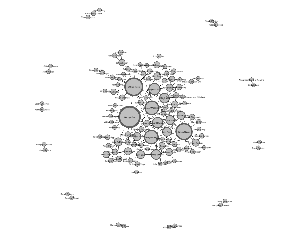Force-directed network visualization of the Quaker data, created in Gephi

There are lots of ways to visualize a network, and a force-directed layout, of which the above image is an example, is among the most common.

除了visualization，看看network density吧. density是网络中实际边与网络中所有可能边的比率。 the best way to do this is to store your metric in a variable for future reference, and print that variable.

density = nx.density(G)
print("Network density:", density)

最短路径

看名字就知道啥意思：A shortest path measurement calculates the shortest possible series of nodes and edges that stand between any two nodes. The Six Degrees of Kevin Bacon game, from which our project takes its name, is basically a game of finding shortest paths (with a path length of six or less) from Kevin Bacon to any other actor.

Let’s find the shortest path between Margaret Fell and George Whitehead:

fell_whitehead_path = nx.shortest_path(G, source="Margaret Fell", target="George Whitehead")
print("Shortest path between Fell and Whitehead:", fell_whitehead_path)
print("Length of that path:", len(fell_whitehead_path)-1) #length of path

这个执行比较费时，因为先要找出所有，在选出最短的。 python还有一些玩shortest path 的工具，如最短路径、全局最短路径、是否存在路径等。请看文档：link diameter: 图中最长的最短路径。用nx.diameter(G)，在Quaker网络里会报错，因为有孤立的边。

找出最大component并生成子图

You can remedy this by first finding out if your Graph “is connected” (i.e. all one component) and, if not connected, finding the largest component and calculating diameter on that component alone. Here’s the code:

# If your Graph has more than one component, this will return False:
print(nx.is_connected(G))

# Next, use nx.connected_components to get the list of components,
# then use the max() command to find the largest one:
components = nx.connected_components(G)
print('num of connected_components:', nx.number_connected_components(G))
largest_component = max(components, key=len)

# Create a "subgraph" of just the largest component
# Then calculate the diameter of the subgraph, just like you did with density.
#

subgraph = G.subgraph(largest_component)
diameter = nx.diameter(subgraph)
print("Network diameter of largest component:", diameter)

Traverse all connected components:

# Traverse all connected components:
# gen the list of components 
compnt_list = []       # list of component, each component is a set
list_componet_size = []   # list of size of each component, list of numbers
for compnt_i in nx.connected_components(G):  # type(compnet_i) = set
    compnt_list.append(compnt_i)
    list_componet_size.append(len(compnt_i))
    print(compnt_i)
compnt_list.sort(key=len, reverse=True)
list_componet_size.sort(reverse=True)
print('list of size of componet (sorted):', list_componet_size)
subgraph = G.subgraph(compnt_list[2]) # create subgraph using the 3-th largest component 

triadic closure

Triadic closure 是指如果2人正好认识同1个人，那么这2个人倾向于互相认识。这回造成三角形的闭环，completing a triangle in the visualization of three edges connecting Fox, Fell, and Whitehead. The number of these enclosed triangles in the network can be used to find clusters and communities of individuals that all know each other fairly well.

计算triadic closure的方法叫clustering coefficient，because of this clustering tendency. 但在这里要用的概念叫Transitivity. Transitivity is the ratio of all triangles over all possible triangles.

You can calculate transitivity in one line, the same way you calculated density:

triadic_closure = nx.transitivity(G)
print("Triadic closure:", triadic_closure)

Quaker网络中的transitivity = 0.1694左右，比density 0.0248 大，说明图不稠密，还有一些possible triangles to begin with. 也说明，那些有更高度数的nodes更倾向于存在在三角形中。也就是说，已经有很多连接的节点很可能是这些封闭三角形的一部分。为了支持这一点，您需要更多地注意具有高度数的节点。 a good next step is to find which nodes are the most important ones in your network.

Centrality

Which nodes are the most important?” there are many different ways of calculating centrality. Here you’ll learn about three of the most common centrality measures: degree, betweenness centrality, and eigenvector centrality.

度数degree

• 最简单直接常用的一个统计量，就是一个节点身上的边的数量。 先创建一个包含degree的dictionary，作为attribute 添加到每个节点中。The keys are nodes and the values are centrality measures.

degree_dict = dict(G.degree(G.nodes()))
nx.set_node_attributes(G, 'degree', degree_dict) #注意参数顺序
print(G.node['William Penn']) #see William Penn’s degree along with his other information 

在你网络的所有节点G.nodes()的列表上，使用G.degree()方法。可看到console输出：

{'historical_significance': 'Quaker leader and founder of Pennsylvania', 'gender': 'male', 'birth_year': '1644', 'death_year': '1718', 'sdfb_id': '10009531', 'degree': 18}

如果你想画出 degree 的分布直方图，参考：draw histogram

在python可以任意sort一些值: 比如使用内建的sourted()函数来sort一个dictionary by its keys or values. 并找到top 20的nodes ranked by degree. 你需要用itemgetter()来帮你搞定。如下：

sorted_degree = sorted(degree_dict.items(), key=itemgetter(1), reverse=True)

看sorted()的三个参数：

• 第一个是 the dictionary you want to sort;
• 第二个是 what to sort by，在这里1是指第2个值，或者是the value of your dictionary;
• 第三个是 要不要Reverse. True -> Highest be the first.降序

建立了sorted list, 就可以loop through it, and use list slicing to get only the top 20 nodes:

print("Top 20 nodes by degree")
for d in sorted_degree[:20]:
    print d

其实你看到的度数高的人，那些hub，如William Penn, 他是 Quaker leader 确实很重要，但多数social networks have just few hubs, 剩下的不那么高的又怎样呢？ 很多时候那些高度数的节点带来的信息并不令人惊奇，比如 Penn or Quakerism co-founder Margaret Fell, with a degree of 13. 你会发现高度数的人基本上就是那些founder.

特征向量中心性 Eigenvector centrality is a kind of extension of degree - 它考虑了本身的度数和它邻居的度数（但不是简单的比例关系，要用$Ax = \lambda x$算）。Eigenvector centrality cares if you are a hub, but it also cares how many hubs you are connected to. 对于了解哪些节点可以快速获取其他节点的信息，Eigenvector centrality就有用了。它被计算为从0到1的值：越接近1，中间度越大。如果你认识很多有关系的人，你可以很有效地传播信息。

介数中心性 Betweenness centrality is a bit different. 介数中心性 doesn’t care about the number of edges any one node. 介数中心性考虑的是所有的shortest paths that pass through a particular node. To do this, it must first calculate every possible shortest path in your network, so keep in mind that betweenness centrality will take longer to calculate than other centrality measures. 介数中心性(也以0到1的尺度表示)在查找连接网络中两个不同部分的节点方面相当出色。如果您是连接两个集群的唯一对象，那么这些集群之间的所有通信都必须经过您。与hub不同，这种节点通常称为broker代理。这个指标不是找到brokerage的唯一方法，还有别的系统化的方法。但它很简单，不是因为它占有边数多，而是它提供了一个不同groups之间的桥梁，cohesion.

These two centrality measures are even simpler to run than degree—they don’t need to be fed a list of nodes, just the graph G. You can run them with these functions:

eigenvector_dict = nx.eigenvector_centrality(G) # Run eigenvector centrality
betweenness_dict = nx.betweenness_centrality(G) # Run betweenness centrality

# Assign each to an attribute in your network
nx.set_node_attributes(G, 'betweenness', betweenness_dict)
nx.set_node_attributes(G, 'eigenvector', eigenvector_dict)

同样可以sort 这些量：

sorted_betweenness = sorted(betweenness_dict.items(), key=itemgetter(1), reverse=True)

print("Top 20 nodes by betweenness centrality:")
for b in sorted_betweenness[:20]:
    print(b)

你可以看到，有高度数的节点通常有高介数中心性，但看看Elizabeth Leavens 和 Mary Penington， 她们的度数分别为：2 & 4, 在top20之外。 介数中心性分别为：0.027(17th) & 0.024(20th)。在Python中进行这些计算的优点是可以快速比较两组计算。如果你想知道介数中心性高的节点中哪个节点度低呢?也就是说:哪些高介数中心性节点是意料之外的?您可以使用以上排序列表的组合:

#First get the top 20 nodes by betweenness as a list
top_betweenness = sorted_betweenness[:20]

#Then find and print their degree
for tb in top_betweenness: # Loop through top_betweenness
    degree = degree_dict[tb[0]] # Use degree_dict to access a node's degree, see footnote 2
    print("Name:", tb[0], "| Betweenness Centrality:", tb[1], "| Degree:", degree)

从这些结果可以证实，有些人，比如Leavens和Penington，中间度高，度低。这可能意味着，这些女性是重要的经纪人，将原本不同的部分联系在一起。你还可以了解到你已经认识的人的一些意想不到的事情——在这个列表中，你可以看到佩恩的degree比贵格会创始人乔治·福克斯低，但中间度更高。也就是说，仅仅认识更多的人并不够。

这只触及了在Python中使用网络度量可以做的事情的表面。NetworkX提供了许多函数和度量，供您以各种组合方式使用，您可以使用Python以几乎无限的方式扩展这些度量。像Python编程语言或者R将给你灵活地探索你的网络计算方式，其他接口不能，通过允许你结合和比较你的网络与其他属性的统计结果数据(如日期和职业，一开始本教程时你就添加到网络了!)。

社区发现

Advanced NetworkX: Community detection with modularity 关于网络数据集的另一个常见问题是，在更大的社会结构中，子组或社区是什么。你的社交网络是一个人人都认识的快乐大家庭吗?或者，它是一组较小的子组，仅由一两个中介连接? 有好多方法，但比较常见的是用modularity来做社区发现。Modularity is a measure of relative density in your network: a community (called a module or modularity class) has high density relative to other nodes within its module but low density with those outside.

Modularity gives you an overall score of how fractious your network is, and that score can be used to partition the network and return the individual communities.

Though we won’t cover it in this tutorial, it’s usually a good idea to get the global modularity score first to determine whether you’ll learn anything by partitioning your network according to modularity. To see the overall modularity score, take the communities you calculated with communities = community.best_partition(G) and run global_modularity = community.modularity(communities, G). Then just print(global_modularity).

Community detection and partitioning in NetworkX requires a little more setup than some of the other metrics. There are some built-in approaches to community detection (like minimum cut, but modularity is not included with NetworkX. Fortunately there’s an additional python module you can use with NetworkX, which you already installed and imported at the beginning of this tutorial. You can read the full documentation for all of the functions the community module offers, but for most community detection purposes you’ll only want best_partition():

communities = community.best_partition(G)

上面代码会创建一个字典，best_partition()要看适合这个graph的最合理的# of communities. 并给每个node assign一个编号，从0开始。就是每个node belong to 的编号。你可以add these values to nodes in the same way:

nx.set_node_attributes(G,'modularity',communities)

你可以把他们结合起来，比如你找找在modularity 0中，最大的eigenvector centrality是哪个Node:

# First get a list of just the nodes in that class
class0 = [n for n in G.nodes() if G.node[n]['modularity'] == 0]

# Then create a dictionary of the eigenvector centralities of those nodes
class0_eigenvector = {n:G.node[n]['eigenvector'] for n in class0}

# Then sort that dictionary and print the first 5 results
class0_sorted_by_eigenvector = sorted(class0_eigenvector.items(), key=itemgetter(1), reverse=True)

print("Modularity Class 0 Sorted by Eigenvector Centrality:")
for node in class0_sorted_by_eigenvector[:5]:
    print("Name:", node[0], "| Eigenvector Centrality:", node[1])

使用特征向量中心性作为排序，可以让您了解这个模块化类中的重要人物。你会注意到，前五名中的大多数人，尤其是William Penn, William Bradford (not the Plymouth founder), and James Logan,都在美国呆了很长时间。Bradford and Tace Sowle都是著名的贵格会印刷商。只要稍加挖掘，我们就会发现，这群人属于一起，既有地理上的原因，也有职业上的原因。这表明模块化可能正在按照预期工作。我想说的是，对于数据的背景理解很重要。

在像这样的小型网络中，一个常见的任务是查找并列出所有模块化类及其成员。在较大的网络中，列表可能长得难以阅读，可以通过可视化网络并根据节点的模块类为其添加颜色。You can do this by manipulating the communities dictionary. You’ll need to reverse the keys and values of this dictionary so that the keys are the modularity class numbers and the values are lists of names. You can do so like this把这个dictionary的keys 和 values对调过来:

modularity = {} # Create a new, empty dictionary
for k,v in communities.items(): # Loop through the community dictionary
    if v not in modularity:
        modularity[v] = [k] # Add a new key for a modularity class the code hasn't seen before
    else:
        modularity[v].append(k) # Append a name to the list for a modularity class the code has already seen

for k,v in modularity.items(): # Loop through the new dictionary
    if len(v) > 2: # Filter out modularity classes with 2 or fewer nodes
        print('Class '+str(k)+':', v) # Print out the classes and their members

In the line if len(v) > 2,我们把包含少于2个节点的modularity滤除了。

单独使用NetworkX将使您走得更远，您可以通过直接使用数据找到关于模块化类的许多信息。但是，您几乎总是希望可视化数据(也许还希望将模块化表示为节点颜色)。在下一节中，您将了解如何导出NetworkX数据以供其他程序使用。

导出数据和做结论

导出数据

NetworkX 支持各种数据格式的导出 for data export. If you wanted to export a plaintext edgelist to load into Palladio, there’s a convenient wrapper for that. Frequently at Six Degrees of Francis Bacon, we export NetworkX data in D3’s specialized JSON format, for visualization in the browser. 如果你有更高级的统计操作，你可以 export your graph as a Pandas dataframe . 有很多选项，如果您一直在努力将所有matrics作为属性添加到图形对象中，那么您的所有数据将一次性导出。

多数格式的导出方法都一样，这里我们 export data into Gephi’s GEXF format. 用它，你可以 upload it directly into Gephi for visualization.通常一句代码就搞定，用 quaker_network.gexf. To export type:

nx.write_gexf(G, 'quaker_network.gexf')

That’s it! When you run your Python script, it will automatically place the new GEXF file in the same directory as your Python file. 每一种可以导出的格式就是可以导入的。 If you have a GEXF file from Gephi that you want to put into NetworkX, you’d type G = nx.read_gexf('some_file.gexf').

结论Draw conclusions

在用Python处理和审查了一系列网络指标之后，您现在有了关于这个早期现代英国教友派信徒网络的争论和结论的证据。例如，您知道网络的密度相对较低，这意味着松散的关联和/或不完整的原始数据。你知道，这个社区是围绕着几个不成比例的大中心hubs组织起来的，其中包括玛格丽特·费尔(Margaret Fell)和乔治·福克斯(George Fox)等教派的创始人，以及威廉·佩恩(William Penn)等重要的政治和宗教领袖。更有帮助的是，你知道一些学历相对较低的女性，比如伊丽莎白•里维斯(Elizabeth Leavens)和玛丽•佩宁顿(Mary Penington)，她们(由于中间度较高)可能充当了中间人brokers，将多个群体联系起来。最后，您了解到网络是由一个大组件components和许多非常小的组件组成的。在这个最大的组成部分中，有几个截然不同的社区communities，其中一些似乎是围绕时间或地点组织起来的(比如佩恩和他的美国同事)。由于您将元数据添加到网络中，因此您可以使用工具进一步研究这些指标，并可能解释您确定的一些结构特性。

每一个发现都是对更多研究的邀请，而不是终点或证据。网络分析是一组关于数据集中关系结构的有针对性问题的工具，NetworkX为许多常用技术和指标提供了一个相对简单的接口。通过提供关于社区结构的信息，网络是将研究扩展到小组的一种有用方式，我们希望您能从本教程中得到启发，使用这些指标来丰富您自己的研究，并探索网络分析的灵活性，而不仅仅是可视化。

这篇tutorial，作者相当的用心啊。全篇浑然一体，简直是教材级的干货~ 入门用，难得的好~精品！