Getting started with Graph Convolutional Networks as an Amateur

https://zhuanlan.zhihu.com/p/27587371

https://www.cnblogs.com/wangxiaocvpr/p/8306519.html

https://www.cnblogs.com/wangxiaocvpr/p/8299336.html

https://towardsdatascience.com/how-to-do-deep-learning-on-graphs-with-graph-convolutional-networks-7d2250723780

GCN是一种强大的神经网络，旨在直接在图上工作并利用其结构信息。这篇文章是关于如何用图卷积网络（GCN）在图上进行深度学习的系列文章的第一篇。该系列的包含：

1. 本篇：一个高层级的GCN介绍
2. 谱图卷积的半监督学习

最基本的代码实现GCN – 一个高层级的GCN介绍

In this post, I will illustrate how information is propagated through the hidden layers of a GCN using coding examples. 看看GCN是如何从前几层聚合信息的，以及这种机制是如何产生图中节点的有用特征表示的。 ref link in Chinese中文

看看GCN的输入是啥

Given a graph $G = (V, E)$ , a GCN takes as input:

• adjacency matrix $\mathbf{A}$ of $G$. N × N
• an input feature matrix, $N × F⁰$ feature matrix, $\mathbf{X}$,
  • where N is the number of nodes and
  • F⁰ is the number of input features for each node

图示是一个例子

对图中示例的解释：

以一个包含4个节点的图为例，圆括号是每个节点的属性信息。有向边（v,n）表示从v->n的边，此时定义n是节点v的邻居。

GCN的隐藏层记作： $H^{i} = f(H^{i-1}, \mathbf{A})$

如果将 $f$ 这个传播规则定义为最简单的 $f(\cdot) = \mathbf{A} \times H^{i-1}$

$$ \mathbf{A} = \begin{bmatrix} 0&1&0&0 \ 0&0&1&1 \0&1&0&0 \1&0&1&0 \ \end{bmatrix} $$

$$ H^{i-1} = \begin{bmatrix} 0&0 \ 1&-1 \ 2&-2 \ 3&-3 \ \end{bmatrix} $$

$$ H^{i} = \mathbf{A} \times H^{i-1} = \begin{bmatrix} 1 & -1 \ 5 & -5 \ 1 & -1 \ 2 & -2 \end{bmatrix} $$

通过一次传播，得到了节点的新的特征$H^i$ .

如果我们还有节点的度矩阵： $D$ ，利用 $D$ 可以对 $H^i$ 进行归一化： $f(X,A) = D^{-1} \mathbf{A} X$ or $f(X,A) = D^{-1} \mathbf{A} H^{i}$

此例中，$$D = \begin{bmatrix} 1&0&0&0 \ 0&2&0&0 \0&0&2&0 \0&0&0&1 \ \end{bmatrix}$$

归一化后，上面的 $H^i$ 变为：$$ H^i = \begin{bmatrix} 1&-1 \ 2.5&-2.5 \ 0.5&-0.5 \ 2&-2 \end{bmatrix} $$

几个问题

**问题1：**该表征是相邻节点的特征聚合， 节点的聚合表征不包含它⾃⼰的特征！只有具有⾃环（self-loop）的节点才会在该聚合中包含⾃⼰的特征。在邻接矩阵A中，对角线上为1的节点才是具有自环的节点。

**问题2：**度⼤的节点在其特征表征中将具有较⼤的值，度⼩的节点将具有较⼩的值。会影响随机梯度下降算法，比如梯度爆炸。

解决：

1. 增加自环，在A中加入eye矩阵 $I$：np.eye(A.shape[0])
2. 对表征进行归一化。如：$f(X,A) = D^{-1} \mathbf{A} X$

2. 整合

这一节要把前面讨论的增加自环、归一化加入，还要加入前面省略的权重和激活函数。

即： 自环 - 归一化 - 权重 - 激活函数

2.1 应用权重

一个定义，添加了自环的adj_Matrix：$\hat{\mathbf{A}} = \mathbf{A} + I$ 。 $D$ 是 $\mathbf{A}$ 的度矩阵，定义$\hat{D}$ 是 $\hat{\mathbf{A}}$ 的度矩阵。

权重矩阵： $$W = \begin{bmatrix} 1&-1 \ -1&1 \end{bmatrix}$$

计算此时的属性传播：$\hat{D}^{-1} \times \hat{\mathbf{A}} \times X \times W$

上面的 $H^i$ 即为：$$ H^{i} = \begin{bmatrix} 1 \ 4 \ 2 \ 5 \end{bmatrix} $$

再用ReLu函数套一下：relu(D_hat**-1 * A_hat * X * W)

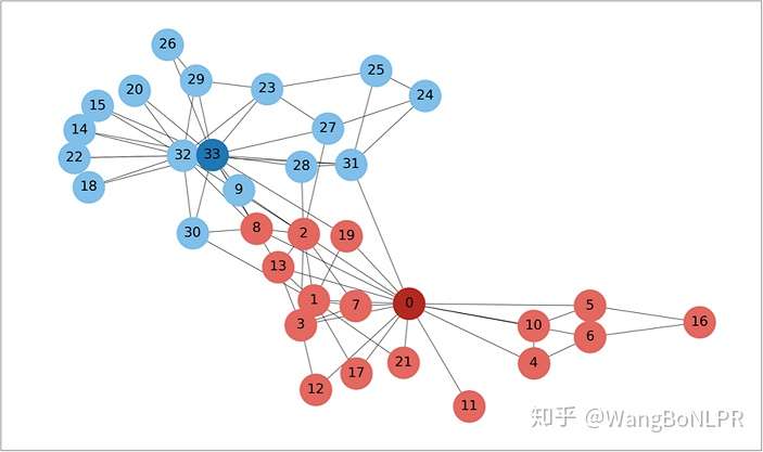
3. 应用于 Karate 网络数据

在 Zachary’s Karate Club 网络上进行GCN

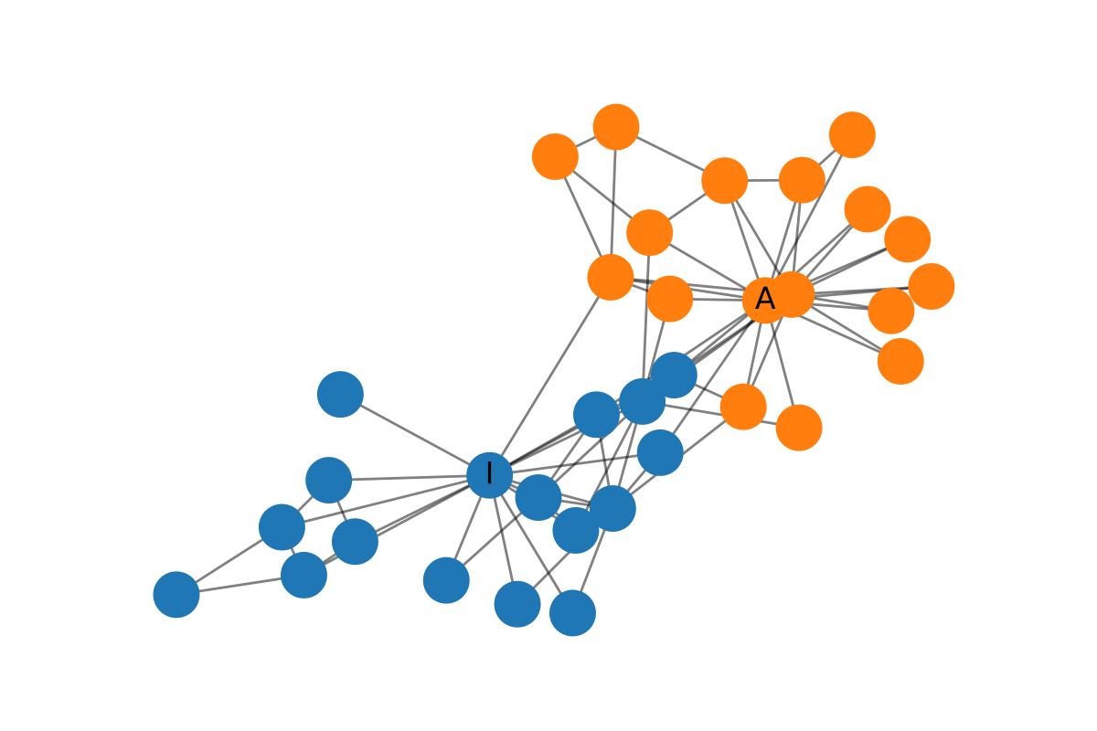
Zachary’s Karate Club:

先随机初始化一把：计算A_hat 和 D_hat 矩阵

# 计算A_hat 和 D_hat 矩阵
from networkx import karate_club_graph, to_numpy_matrix
zkc = karate_club_graph()
order = sorted(list(zkc.nodes()))  # order = [0,1,2,...]

A = to_numpy_matrix(zkc, nodelist=order)   # 输入一个nx.graph, this shows 如何生成它的 adj_Matrix
I = np.eye(zkc.number_of_nodes())
A_hat = A + I
D_hat = np.array(np.sum(A_hat, axis=0))[0]
D_hat = np.matrix(np.diag(D_hat))

# initialize the weights randomly
W_1 = np.random.normal(loc=0, scale=1, size=(zkc.number_of_nodes(), 4))   # W1: shape: (34,4)
W_2 = np.random.normal(loc=0, size=(W_1.shape[1], 2))  # W2 shape: (4,2)

Stack the GCN layers.

We here use just the identity matrix as feature representation, that is, each node is represented as a one-hot encoded categorical variable.

feature representation will be like:

node_0: 1,0,0,...,0
node_1: 0,1,0,...,0
node_2: 0,0,1,0,..,0
...

# Each transmit is a layer, so defines it as a function
def gcn_layer(A_hat, D_hat, X, W):
    return relu(D_hat**-1 * A_hat * X * W)

# H1 <= A_hat + D_hat + H_0(I) + weight(W_1)
H_1 = gcn_layer(A_hat, D_hat, I, W_1)     # note the I here: I = np.eye(zkc.number_of_nodes())

# H2 <= A_hat + D_hat + H_1 + W_1
H_2 = gcn_layer(A_hat, D_hat, H_1, W_2)

output = H_2

# We extract the feature representations.
feature_representations = {
    node: np.array(output)[node] 
    for node in zkc.nodes()}

feature_representations

{0: array([0.27514556, 0.2916475 ]),
 1: array([0.23384102, 0.12333202]),
 2: array([0.10573154, 0.19859599]),
 3: array([0.10044765, 0.15261897]),
 4: array([0.23252655, 0.68635458]),
 5: array([0.41926146, 1.2925271 ]),
 6: array([0.45833935, 1.42640262]),
 7: array([0.06380073, 0.13444717]),
 8: array([0.17890381, 0.37274954]),
 9: array([0.12122856, 0.20078968]),
 10: array([0.23332865, 0.6970111 ]),
 11: array([0.42113657, 0.21505439]),
 12: array([0.17455961, 0.33643646]),
 13: array([0.10565966, 0.20771884]),
 14: array([0.33195037, 0.53988095]),
 15: array([0.49140489, 1.08604872]),
 16: array([0.60948432, 1.93432754]),
 17: array([0.43220848, 0.29479237]),
 18: array([0.28285175, 0.55598298]),
 19: array([0.17600684, 0.31744565]),
 20: array([0.33020733, 0.73801137]),
 21: array([0.36867983, 0.3119505 ]),
 22: array([0.34193455, 0.50004196]),
 23: array([0.46985141, 0.7935709 ]),
 24: array([0.79867382, 1.25776893]),
 25: array([0.81112201, 1.25608014]),
 26: array([0.13385231, 0.19571042]),
 27: array([0.47025238, 0.76962093]),
 28: array([0.1175102 , 0.15650574]),
 29: array([0.23946535, 0.42422421]),
 30: array([0.1985622 , 0.32838823]),
 31: array([0.5660882 , 0.98039276]),
 32: array([0.18968005, 0.30977425]),
 33: array([0.15852075, 0.25247645])}

# visualize the feature
import matplotlib.pyplot as pltt

def plot_embeddings(M_reduced, word2Ind, words):
    """ 
        Plot in a scatterplot the embeddings of the words specified in the list "words".
        Include a label next to each point.
    """
    for word in words:
        x, y = M_reduced[word2Ind[word]]
        pltt.scatter(x, y, marker='o', color='red')
        pltt.text(x+.006, y+.006, word, fontsize=9)
    pltt.show()

"""
M_reduced_plot_test = np.array([[1, 1], [-1, -1], [1, -1], [-1, 1], [0, 0]])
word2Ind_plot_test = {'test1': 0, 'test2': 1, 'test3': 2, 'test4': 3, 'test5': 4}
words = ['test1', 'test2', 'test3', 'test4', 'test5']
plot_embeddings(M_reduced_plot_test, word2Ind_plot_test, words)

"""

N = len(feature_representations)
M_reduced_plot = np.stack([feature_representations[key_i] for key_i in feature_representations])
word2Ind_plot = {}
words = []
for i in range(N):
    label_i = str(i)
    word2Ind_plot[label_i] = i
    words.append(label_i)

plot_embeddings(M_reduced_plot, word2Ind_plot, words)

    

这个结果看起来还是不够直观，常常遇到x坐标为零，或者y坐标为零。 在这个例子中，随机初始化的权重很可能因为ReLU函数而在x轴或y轴上给出0值，所以需要随机初始化几次才能产生上图。

总结

在这篇文章中，我对图卷积网络进行了高层次的介绍，并说明了GCN中每一层的节点的特征表示是如何基于其邻域的集合的。我们看到了如何使用numpy构建这些网络，以及它们有多么强大：即使是随机初始化的GCN也能在Zachary的空手道俱乐部中分离出社区。 在下一篇文章中，我将对技术细节进行深入探讨，并展示如何使用半监督学习实现和训练一个最近发表的GCN。你可以在这里找到这个系列的下一篇文章。 喜欢你读的东西吗？可以考虑在Twitter上关注我，除了我自己的文章之外，我还会分享与数据科学和机器学习的实践、理论和伦理学有关的论文、视频和文章。 有关专业咨询，请在LinkedIn上联系我，或在Twitter上直接留言。

参考下一节： Part 2: Semi-Supervised Learning with Spectral Graph Convolutions